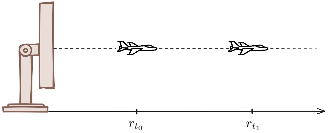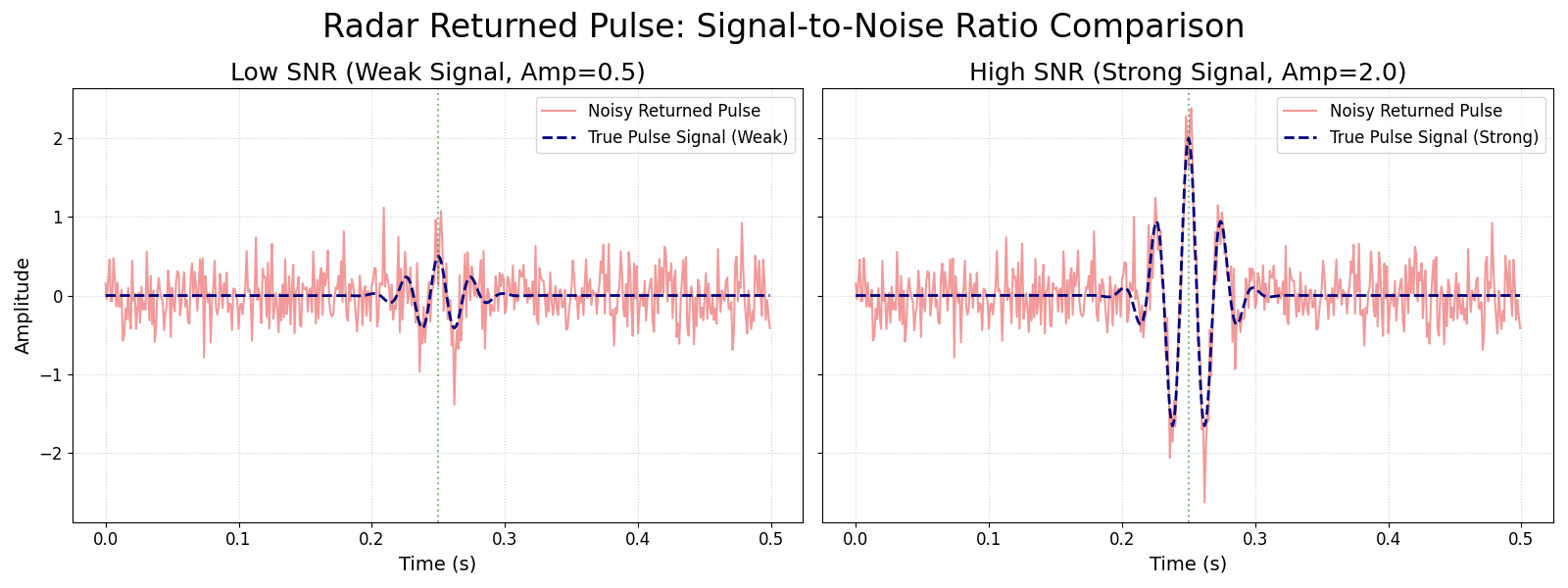
The Kalman filter stands out as one of the most reliable tools for extracting signal from noise in dynamic systems. Engineers and quants use it daily to track everything from missiles to market prices. A Hacker News post breaks it down with a radar tracking an airplane—position unknown, measurements noisy. This matters because real-world data is always messy: sensors glitch, markets jump, crypto charts spike. Get the state right, and you predict; screw it up, and you chase ghosts.
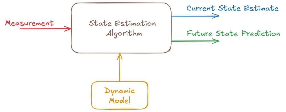
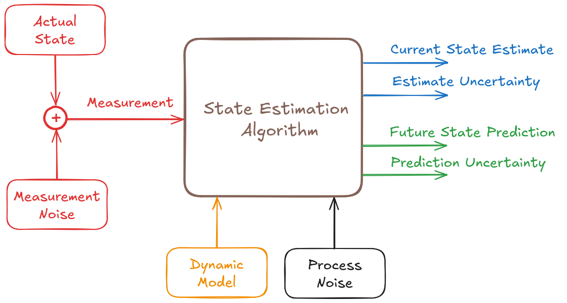
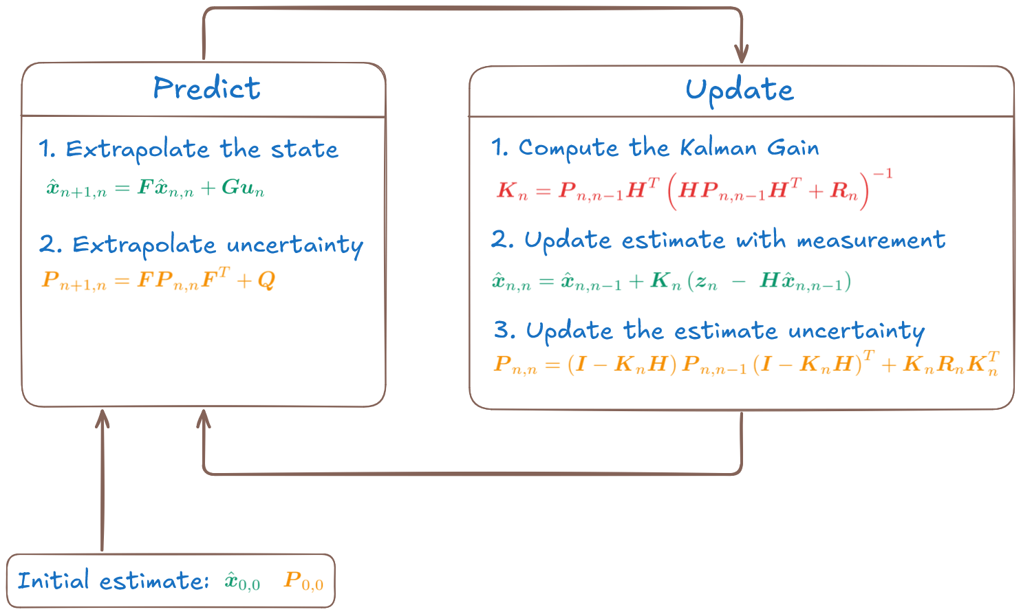
Invented in 1960 by Rudolf Kalman, the filter assumes linear dynamics and Gaussian noise. It runs two steps: predict the next state based on a model, then update with new measurements. The magic is in the weights—it balances trust between your prediction (how well your model holds) and the observation (how accurate your sensor is). Quantitatively, it minimizes the mean squared error via covariance matrices. No hand-waving: the gain K is K = P H^T (H P H^T + R)^{-1}, where P tracks prediction uncertainty, H maps state to measurement, and R is measurement noise.
Radar Example: Tracking a Plane
Picture a radar station at (0,0) pinging a plane flying straight at constant velocity. State vector: [x, vx, y, vy]—position and speed in 2D. Radar measures range r = sqrt(x^2 + y^2) and bearing θ = atan2(y,x), both corrupted by noise, say 10m range error and 0.1 rad angle noise.
Without filter: Plot raw ranges, and the path zigzags wildly. Prediction step extrapolates: x_new = F x, where F is the transition matrix (identity plus time-scaled velocities). Uncertainty grows via P_new = F P F^T + Q, Q process noise.
Update fuses: Innovation y = z - H x (measurement minus predicted). Adjust state x = x + K y. In the HN example, after 20 pings, filtered track hugs the true path while raw data scatters. Skeptical note: This shines for linear Gaussian cases. Radar range is nonlinear—real ops use Extended Kalman Filter (EKF), linearizing around the estimate. EKF works but diverges if nonlinearity bites hard.
import numpy as np

# Simple 1D position-velocity tracker
dt = 1.0
F = np.array([[1, dt], [0, 1]])  # State transition
H = np.array([[1, 0]])          # Measurement matrix (position only)
Q = np.eye(2) * 0.1             # Process noise
R = 1.0                         # Measurement noise

def kalman_update(x, P, z):
    y = z - H @ x
    S = H @ P @ H.T + R
    K = P @ H.T / S
    x = x + K.flatten() * y
    P = (np.eye(2) - K @ H) @ P
    return x, P

# Simulate: true pos=10t, v=2, noisy z=10t+2 + N(0,1)
x = np.zeros(2)
P = np.eye(2)
for t in range(20):
    z = 10*t + 2 + np.random.normal(0,1)
    x, P = kalman_update(x, P, z)
    print(f"t={t}: est={x[0]:.2f}")
This Python snippet converges fast—estimates nail truth despite noise. Scale to radar: Stack x/y states, nonlinearize H.
Why This Matters in Tech, Finance, Crypto
Beyond radar, Kalman filters power GPS (fuses IMU, satellites), self-driving (tracks cars from lidar/camera), and drones. In finance, quants apply it to pairs trading: estimate cointegration between stocks amid volatility. Example: Track Bitcoin-Ethereum spread. Crypto exchanges spew tick data with lags, wash trades—filter smooths for arb signals.
Security angle: Anomaly detection in network traffic. Model normal flows; filter flags deviations as attacks. High-frequency trading desks run variants for order book state. A 2022 study by Jump Trading cited Kalman-inspired filters cutting latency prediction error by 30%.
Fair caveat: It fails on fat tails (crypto crashes) or regime shifts (flash crashes). Switch to particle filters or LSTMs then. But for 80% of tracking jobs, Kalman is zero-fuss optimal. The HN post nails accessibility—run the sim, see the filter pull order from chaos. In a noisy world, that’s gold.